Flow reconstruction from sparse sensors.
Pi-LNN combines DeepONet operator learning with CfC (closed-form continuous-time) memory to reconstruct a Re = 10,000 two-dimensional Kolmogorov flow from only K = 100 velocity sensors. The model never sees a full DNS field — its supervision is pointwise sensor MSE plus the residual of the Navier–Stokes equations.
A real engineering sensor scene, reconstructed by physics alone.
We take the engineering scenario seriously: only point-wise velocity samples are available, and the only auxiliary signal is the governing PDE. Full DNS fields are used offline as a benchmark — never as supervision.
-
- Flow
- Two-dimensional Kolmogorov turbulence on a strict periodic [0, 1]² domain.
-
- Reynolds
- Re = 10,000.High-Re regime with a wide inertial range and rich small-scale vortices.
-
- DNS reference
N = 256,T = 201snapshots,dt = 0.025.Used only to extract sensor values and for offline diagnostics. -
- Forcing
fx = A sin(2π kf y),A = 0.1,kf = 2. -
- Observation
K = 100sensors (QR-pivot placement), velocity componentsu, vonly.Pressurepis unobserved and emerges as an internal physics field. -
- Training signal
- Sensor MSE + NS momentum + continuity residual. Nothing else.
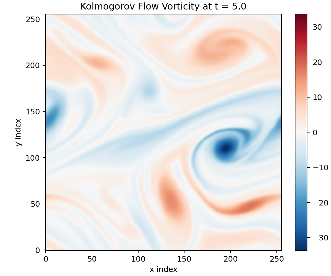
t = 5.0. The model never trains on this field
— it is the offline yard-stick against which every reconstruction figure below is measured.
Two parallel paths, fused in a DeepONet-style readout.
A branch path turns the sensor stream into a continuous-time memory; a
trunk path lifts each query (x, y, t) into an aligned condition
feature. Cross-attention fuses them into a field value.
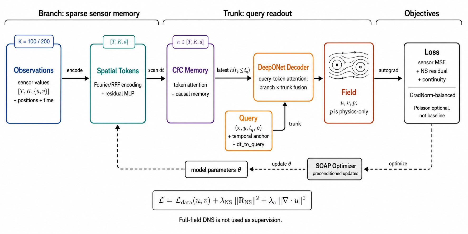
(x, y, t) with a temporal anchor; the DeepONet decoder fuses them and emits
(u, v, p). Training loss is sensor MSE plus NS momentum and continuity
residuals; SOAP applies the preconditioned update. Full-field DNS is used only offline.
Diagram errata: the third branch block reads “CIC Memory” — should be
CfC Memory (closed-form continuous-time). A clean re-render is queued.
d = 128 → SpatialSetEncoder → token attention →
CfC(dt) causal state, yielding a dt-aware token bank.
(x, y, t) with temporal anchor of tq;
shares the same d = 256 latent space as the branch tokens.
= 256; output (u, v, p),
with p recovered from the NS residual.
Want the full graph?
Component-by-component nodes, time semantics, decoder zoom-in, and the closed-form CfC update are documented in the detailed architecture page.
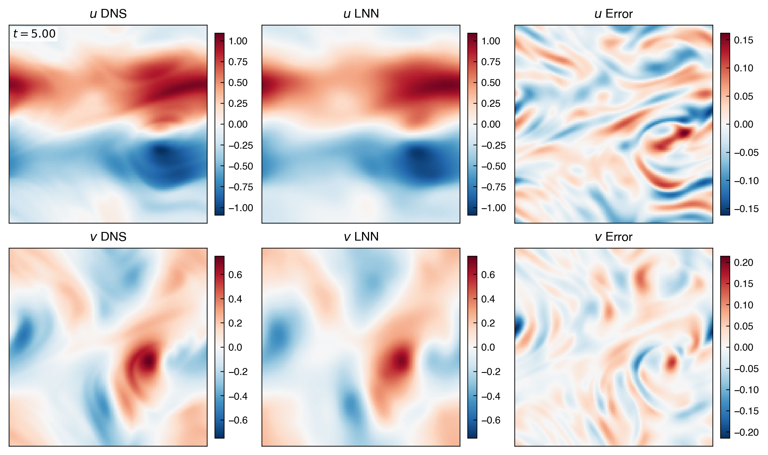
Re = 10,000 reconstruction quality from K = 100.
Field structure, spectral content, and physics constraints are evaluated on the full
T = [0, 5] window. Numbers are versus DNS; the model has not seen any of these
full fields during training.
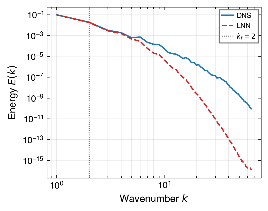
K = 100 is a mathematical ceiling, not an optimisation gap.
The Re = 10,000 velocity field is highly sparse in a db4 wavelet basis (Gini ≈ 0.983). Compressed-sensing theory requires M ≥ O(s · log N) ≈ 5,000 sensors for exact recovery. K = 100 is short by a factor of ~50.
| Frequency band | Energy share | Wavelet DOF | Feasible at K = 100? | EXP-064 band err. |
|---|---|---|---|---|
| Low (k ≤ 8) | 94.4 % | ~196 | Underdetermined — feasible | 3.62 % |
| Mid (8 < k ≤ 16) | 4.8 % | ~588 | Exceeds capacity | ≈ 100 % |
| High (16 < k ≤ 32) | 0.8 % | ~1,452 | Far exceeds capacity | ≈ 100 % |
Convergent evidence — the wall is real
Three independent turbulence-aware variants (multi-scale CfC time-constants, frequency-tiered Fourier, PINN causal weighting; EXP-067 / 068 / 069) all fail to break the mid- and high-band errors. KE regresses by +1.9 to +12.3 percentage points; the band-mid error stays ≈ 100 %. EXP-064 (K = 100, KE 7.80 %) is the global optimum under the current architecture configuration. Further progress requires either more sensors (K ≥ 5,000) or a physical prior that is, by construction, engineering-non-transferable.
Read deeper, run it yourself, or follow the experiment chain.
Detailed architecture
Component-by-component nodes, time semantics, decoder internals, training-loss design, and the closed-form CfC update.
Source code
PyTorch implementation, configs, training scripts, and the evaluation pipeline used for every figure on this page.
Experiment log
Linear chronicle of every run from EXP-001 through the K = 100 ceiling, including hypothesis, falsifying evidence, and post-mortems.